Statistical Rethinking is a fabulous course on Bayesian Statistics (and much more). Following its presentation, I’ll give a succinct intuitive introduction to Gaussian Process (GP) regression as a method to extend the varying effects strategy to continuous predictors. This method is incredibly useful when assuming a linear functional relationship between a continuous predictor and the outcome variable is not enough to capture the variation in the data.
First, I’ll begin by motivating the varying effects strategy. Secondly, I’ll show the intuitive problems of naively extending it to continuous predictors. Thirdly, I’ll show intuitively how the Gaussian Process (GP) regression takes into account these problems when faced with a continuous category. Finally, I’ll show an example of GP regression with simulated data using stan.
Varying Effects Strategy
The varying effects strategy consists in estimating a unique parameter for each cluster in the data as coming from a common distribution. This, in turn, allows us to pool information across clusters whose end result is to shrink our predictions toward the common distribution’s mean. The amount of shrinkage, then, will itself be learnt from the data. Here is a blogpost I wrote trying to understand this fundamental idea.
We can extend this idea by letting different parameter types vary by cluster. For example, an intercept and a slope. Then, we can model them (every pair of intercept and slope) as coming from a common multivariate distribution. The covariance in this distribution will let us pool not only across clusters but also across parameter types. Here is another blogpost of mine where I simulated data to understand how this works.
Naively extending it ignores covariances
Notice that so far we only vary the effects across discrete, exchangeable values that represent different clusters. For example, across classrooms in a school. There’s no meaningful order in the indices: classroom 1 and classroom 2 are just labels.
However, with a continuous variable there’s an order. For example, different ages: 20 years old, 21 years old and 80 years olds have an internal order with specific distances among them (i.e., the age difference); they are, unlike our clusters, not exchangeable. Therefore, were we to estimate a unique parameter for each possible age as coming from a joint distribution, we would be saying that 40 years olds should inform our estimate of the 20 years olds just as much 21 year olds. This is clearly not a good idea: the varying effects strategy should take into account the distance between the ages to determine how much information is pooled across different ages. The closer the ages, the more information we should pool among them; the farther they are, the less we should pool.
Covariances as function of distances
GP regression does precisely this. For example, continuing with the age example, Gaussian Process regression varies the effect of age for each unique age value in the sample such that the observations with similar ages have similar estimated effects. The heart of the method lies in positing a multivariate normal prior for each unique age effect and explicitly modelling the covariance among these effects as a function of the distance between the ages. In math:
\[ \begin{bmatrix} \mu_1 \\ \mu_2 \\ \cdots \\ \mu_N \end{bmatrix} = MultiNormal(\begin{bmatrix} 0 \\ 0 \\ 0 \\ 0 \end{bmatrix}, K) \]
Where \(K\) is the covariance matrix between each observation’s unique age effect. The covariances are modeled as function of the ages’ distance with a kernel function:
\[ K_{ij} = \eta^2 \text{exp}(-\rho^2 D^2_{ij}) \]
Where \(D_{ij}\) is the age difference between the observations. Thus, the covariance between two unique age effects exponentially decreases with the distance between the ages. Therefore, we will pool much more for individuals with similar ages and pool much less for individuals with wider age gaps. Indeed, this is the key to avoid overfitting to the data. This is done through two parameters: \(\eta, \rho\). \(\eta\) controls how strong the covariances between observations can be; \(\rho\) controls how quickly the covariances can change. As usual with bayesian estimation, we’ll have a posterior distribution for both of them.
Notice that this varying effects strategy to each unique age value, whilst modeling the covariance between these unique effects, is equivalent to defining a functional relationship between age and the outcome variable at any age. Indeed, for any unseen age, we just let the covariances between all the seen ages’ effects (and the age gap to this new value) determine what should be the effect for this new unique value of age. That is, each unique value of \(\eta, \rho\) defines a unique functional relationship between age and the outcome variable. Therefore, setting a Gaussian Process is equivalent to setting up a prior over infinitely different functions for the overall functional relationship between age and the outcome variable.
This is the reason why Gaussian Process regression is so useful. We do not prefer a linear or quadratic functional relationship for the relationship between an outcome variable and a continuous predictor. We let the data decide which functional relationship is the most consistent with the data.
GP Regression: simulated cohort voting for two regions
The simulation
Let’s check how these ideas work in practice with a simulated example. This will be loosely based on a paper by Andrew Gelman et alter. Imagine you are modeling cohort voting. Therefore, you are trying to estimate the probability of people voting for the democratic party given their age. Intuitively, individuals with similar ages experienced the same events at the same preference defining moments and were therefore shaped by them in the same way. However, for different cohorts, the events that shaped them were different. Thus, some cohorts are biased towards voting for the democratic party, whilst others the opposite.
To make things a bit more interesting, there is a division in the data from two different regions. This means that the cohort effect varies by region. Although they experienced the same events in both regions, in the north some events were seen favorable whereas in the south the events may be seen negatively. Therefore, we will posit two different Gaussian Processes for each of the regions.
Here, I simulate the (two) GPs to determine the probability of voting for the democratic party for any given age with stan. The code is slightly altered from Michael Betancourt’s excellent post about Gaussian processes. Then, we simulate 5000 bernoulli r.v. according to these probabilities for each region. The stan code is the following:
writeLines(readLines("logit_sim_regions.stan"))##
## data {
## int<lower=1> N_north;
## int<lower=1> N_south;
## real x_north[N_north];
## real x_south[N_south];
##
## real<lower=0> rho_north;
## real<lower=0> rho_south;
## real<lower=0> eta_north;
## real<lower=0> eta_south;
## }
##
## transformed data {
## matrix[N_north, N_north] cov_north = cov_exp_quad(x_north, eta_north, rho_north)
## + diag_matrix(rep_vector(1e-10, N_north));
## matrix[N_north, N_north] L_cov_north = cholesky_decompose(cov_north);
##
## matrix[N_south, N_south] cov_south = cov_exp_quad(x_south, eta_south, rho_south)
## + diag_matrix(rep_vector(1e-10, N_south));
##
## matrix[N_south, N_south] L_cov_south = cholesky_decompose(cov_south);
##
## }
##
## parameters {}
## model {}
##
## generated quantities {
## vector[N_north] f_north = multi_normal_cholesky_rng(rep_vector(0.5, N_north), L_cov_north);
## vector[N_north] y_north;
##
## vector[N_south] f_south = multi_normal_cholesky_rng(rep_vector(-0.5, N_south), L_cov_south);
## vector[N_south] y_south;
##
## for (n in 1:N_north) {
## y_north[n] = bernoulli_logit_rng(f_north[n]);
## }
##
## for (n in 1:N_north) {
## y_south[n] = bernoulli_logit_rng(f_south[n]);
## }
##
## }We’ll simulate with the following parameters for the two different gaussian processes:
eta_true_south <- 0.5
rho_true_south <- 10

eta_true_north <- 2.2
rho_true_north <- 1.5
Notice the different combination of parameters between regions. For the south, the maximum covariance is much smaller as a result of the smaller \(\eta\). Also, the covariances will “wiggle” much less in the south as a result of the larger \(\rho\).
The results of the simulation are two different GP to determine the probability of voting for the democratic party at every possible age:

Notice that in both regions there’s a non-linear effect of age. However, the cohort effects vary much more in the north. This is a direct result of the lower \(\rho\) that we used to simulate the data. These different cohort effects across regions appear partially in our data thus:

Naive multilevel model
A naive way to model this data would be to create a multilevel model where we model a region-specific intercept and a region specific slope for age. However, this would not take into account the highly non-linear responses to age across different cohorts, as it assumes a monotonic relationship between age and the probability of voting democrat. We can code this model thus:
model_naive <- ulam(
  alist(
    vote_dem ~ bernoulli(p),
    logit(p) <- intercept[region] + age_slope[region]*age,
    c(intercept, age_slope)[region] ~ multi_normal(c(a, b), Rho, sigma_region),
    a ~ normal(0, 1),
    b ~ normal(0, 1),
    sigma_region ~ exponential(1),
    Rho ~ lkj_corr(2)
  ),
  data = data_model, chains = 4, cores = 4,
  iter = 2000, log_lik = TRUE
)
Let’s check the posterior’s implied cohort effects against the original GP using the great tidybayes package:
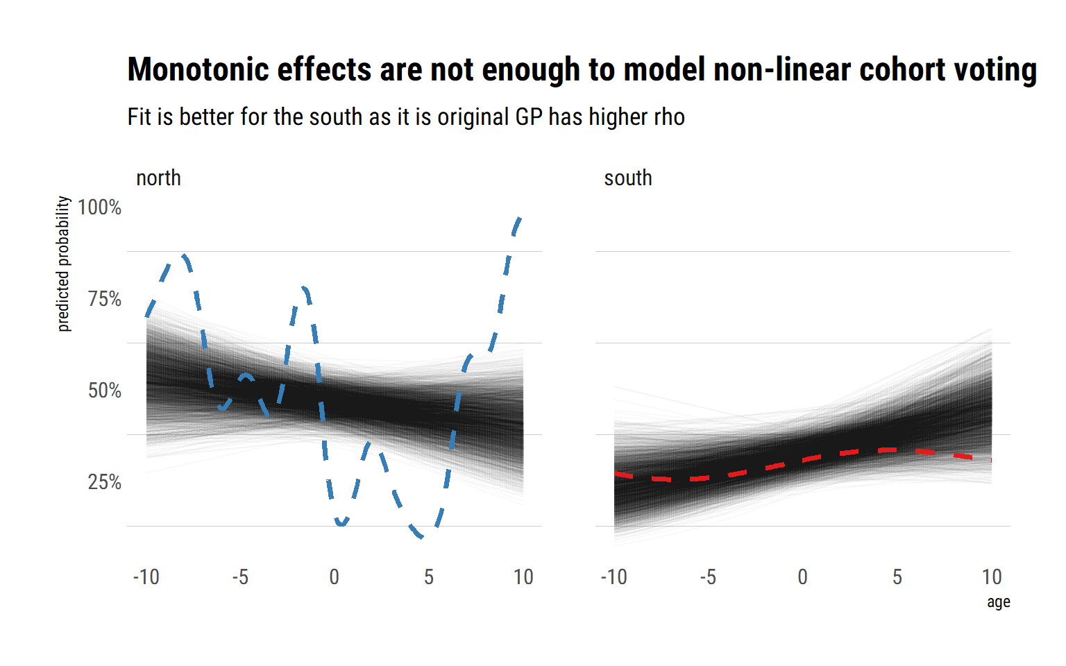
As expected, this naive model does not capture the highly non-linear cohort voting effects present in the data. That is, the fit is too general; we should let the effect of age on the probability of voting for the democratic party vary more across each unique age value. A possible answer would be to include square and cubic terms of age (and quartic, and … where to stop?) in the linear model. However, that is very likely to result in overfitting for the south. Then, we would have to let the linear, square and cubic terms vary by region? This strategy’s complexity is growing more and more. It is just neither scalable nor reliable. A cleaner answer is to let the influence of age on the probability of voting for the Democrats vary by each unique age and region. That is, we must extend the varying effects strategy to include a continuous predictor.
Positing two Gaussian processes
A better strategy than the naive multilevel model is to use two different Gaussian Processes (one for each region) to vary the cohort effects by age. Notice that by letting the effect vary by age and constraining the amount of pooling across of observations by their age gap, we are letting the data specify the functional relationship of cohort voting for each region. Instead of stating a pre-specified functional relationship, we let the data find the best functional relationship by modeling the covariance between each unique age-specific effect.
Our first step, then, is to set up two different age distance matrices: one for the north, other for the south.
distance_matrix <- function(x) {

  matrix_distance <- matrix(nrow = 200, ncol = 200)

  for (row in 1:length(x)) {
    for (col in 1:length(x)) {
      matrix_distance[row, col] = abs(x[row] - x[col])
    }
  }
  matrix_distance
}

simulated_for_model %>%
  filter(region_int == 1) %>%
  pull(age) %>%
  distance_matrix() -> dist_north

simulated_for_model %>%
  filter(region_int == 2) %>%
  pull(age) %>%
  distance_matrix() -> dist_south
Finally, to extend the varying effects strategy it’s a matter of simply setting up a unique parameter for each combination of age value and region, and let the modeling of the covariances do the rest. Using rethinking::ulam we can fit the two Gaussian Processes for both regions (with non centered parametrizations) thus:
model_gps <- ulam(
  alist(
    vote_dem ~ bernoulli(p),
    logit(p) <- intercept[region] + (2-region)*k_north[age_id] + (region - 1)*k_south[age_id],
    # north gp
    transpars> vector[200]:k_north <<- L_SIGMA_north *z,
    vector[200]: z ~ normal(0, 1),
    transpars> matrix[200, 200]: L_SIGMA_north <<- cholesky_decompose(SIGMA_north),
    transpars > matrix[200, 200]: SIGMA_north <- cov_GPL2(dist_north, etasq_north, rhosq_north, 0.01),
    # south gp
    transpars> vector[200]:k_south <<- L_SIGMA_south *z_s,
    vector[200]: z_s ~ normal(0, 1),
    transpars> matrix[200, 200]: L_SIGMA_south <<- cholesky_decompose(SIGMA_south),
    transpars > matrix[200, 200]: SIGMA_south <- cov_GPL2(dist_south, etasq_south, rhosq_south, 0.01),
    # priors
    intercept[region] ~ normal(0, 1),
    c(etasq_north, etasq_south) ~ exponential(0.5),
    c(rhosq_north, rhosq_south) ~ exponential(0.5)
  ), data = data_model, chains = 4, cores = 4, iter = 200, log_lik = TRUE,
  sample = FALSE
)
Let’s check the posterior’s implied cohort effects against the original Gaussian Processes from which we sampled:
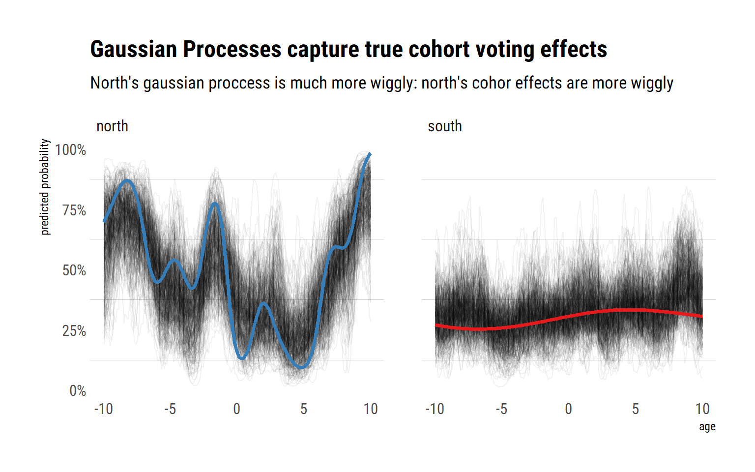
Indeed, by letting each unique age value have a unique influence on the probability of voting democratic, and modeling the covariances between these effects, we have achieved a much better fit with respect to the true cohort effects. This is specially true for the cohort voting effects in the north. That is, GP regression is more useful when the underlying functional relationship between the predictor and outcome variable is highly non-linear.
An alternative way to visualize the different cohort effects across regions is to plot the posterior of the different covariance functions for each respective Gaussian Process. That is, we can visualize how quickly the covariances decrease in both regions. For the north, we expect the covariances to very quickly decrease to zero: this is why we can predict such different age effects for the different cohorts.
 Finally, we can also compare the predictive accuracy out of sample using information criteria for both the naive model and the model using Gaussian Processes:
| model | WAIC | SE | dWAIC | dSE | pWAIC | weight |
|---|---|---|---|---|---|---|
| model_gps | 508.16 | 14.20 | 0.00 | NA | 19.89 | 1.00 |
| model_naive | 529.14 | 10.88 | 20.99 | 9.96 | 4.30 | 0.00 |
Indeed, we gain a lot of predictive accuracy by positing a unique effect for each unique age value and region combination. Even if we are creating around extra 400 parameters, we are not overfitting to the data. This is possible by virtue of modeling the covariances across the different age values’ unique effects as a function of the distance between the ages.
Conclusion
Gaussian Process Regression is a way to extend the varying effects strategy to continuous predictors. We do this by modeling the influence of each unique value in the continuous predictor with its own effect and simultaneously modeling the covariance of these unique effects as a function of the distance between the values in the continuous predictor scale. This is equivalent to let the data model the functional relationship between the continuous predictor and the outcome variable. Therefore, this is incredibly useful when assuming a functional linear relationship is not enough.