I have recently been exploring Nassim Taleb’s latest technical book: Statistical Consequences of Fat Tails. In it, we have seen how the Law of Large Numbers for different estimators simply does not work fast enough (in Extremistan) to be used in real life. For example, we have seen how the distribution of the sample mean, PCA, sample correlation and \(R^2\) turn into pure noise when we are dealing with fat-tails.

In this post, I’ll try to show the same problem for the Central Limit Theorem (CLT). That is, when dealing with fat-tailed random variables with finite variance, the CLT takes way too long to warrant its use. The pre-asymptotic’s behavior, where we live and analyze data, will shows us how different Mediocristan is from Extremistan.

CLT Refresher

You have \(n\) independent and identically distributed random variables. That is: \(X_i\) such that: \(E(X_i) = \mu\) and \(Var(X_i) = \sigma^2 < +\infty\). The CLT tells you that their sample average, \(\bar{X_n}\), as \(n \to \infty\), converges in distribution to a Gaussian:

\[ \sqrt{n}(\bar{X_n} - \mu) \xrightarrow[]d{} N(0, \sigma^2) \]

Which is equivalent to say that the \(Z\)-scores of the sample mean will approximate a standard normal distribution. That is:

\[ \dfrac{\bar{X_n} - \mu}{\sigma{\sqrt{n}}} \xrightarrow[]d{} N(0, 1) \]

Simulating Means

Therefore, if we want to simulate this convergence, we have to evaluate the distribution of the sample mean at different sample sizes. Here’s the code I wrote:

sample_mean <- function(FUN, n) {
  samples <- FUN(n)
  mean(samples)
}

distribution_sample_mean <- function(FUN, n, montecarlo_n) {
  name <- glue::glue("sample_{n}")
  rerun(montecarlo_n, sample_mean(FUN, n)) %>% 
    map(data.frame) %>% 
    bind_rows() %>% 
    rename(!!quo_name(name) := ".x..i..")
}

simulate_sample_means <- function(FUN, montecarlo_n, sample_sizes) {
  map_dfc(sample_sizes, ~ distribution_sample_mean(FUN, .x, montecarlo_n)) %>% 
  cbind(sims = 1:montecarlo_n) %>% 
  pivot_longer(-sims, names_to = "samples_sizes", values_to = "value") %>% 
  mutate(samples_sizes = str_extract(samples_sizes, "\\d+"),
         samples_sizes = as.numeric(samples_sizes))
}

The fastest CLT: Standard Uniform

For example, let’s evaluate the distribution of the sample mean for a Standard Uniform with \(n = 2, 5, 10, 20, 30, 50, 100, 1,000, 10,000\). We will do so by calculating the z-scores of the sample mean and comparing it to a normal distribution, both by comparing densities and with \(QQ\)-plot:

ns <- c(2, 5, 10, 20, 30, 50, 100, 1000, 10000)

uniform <- simulate_sample_means(runif, 3000, ns) %>% 
  rename(uniform = value) %>% 
  group_by(samples_sizes) %>% 
  mutate(z = (uniform - 0.5)*sqrt(12*samples_sizes)) %>% 
  ungroup() %>% 
  mutate(samples_sizes = factor(samples_sizes, ordered = TRUE))

uniform %>% 
  ggplot(aes(sample = z, color = samples_sizes)) +
  stat_qq(alpha = 0.4) +
  stat_qq_line(aes(group = NA)) +
  theme(legend.position = "bottom")  +
  transition_states(samples_sizes) +
  enter_fade() +
  exit_shrink() +
  labs(subtitle = "Sample size {closest_state}",
       title = "Distribution of Sample Mean: Standard Uniform",
       caption = "Theoretical distirbution is standard normal",
       y = "Sample mean from Uniform") +
  view_follow()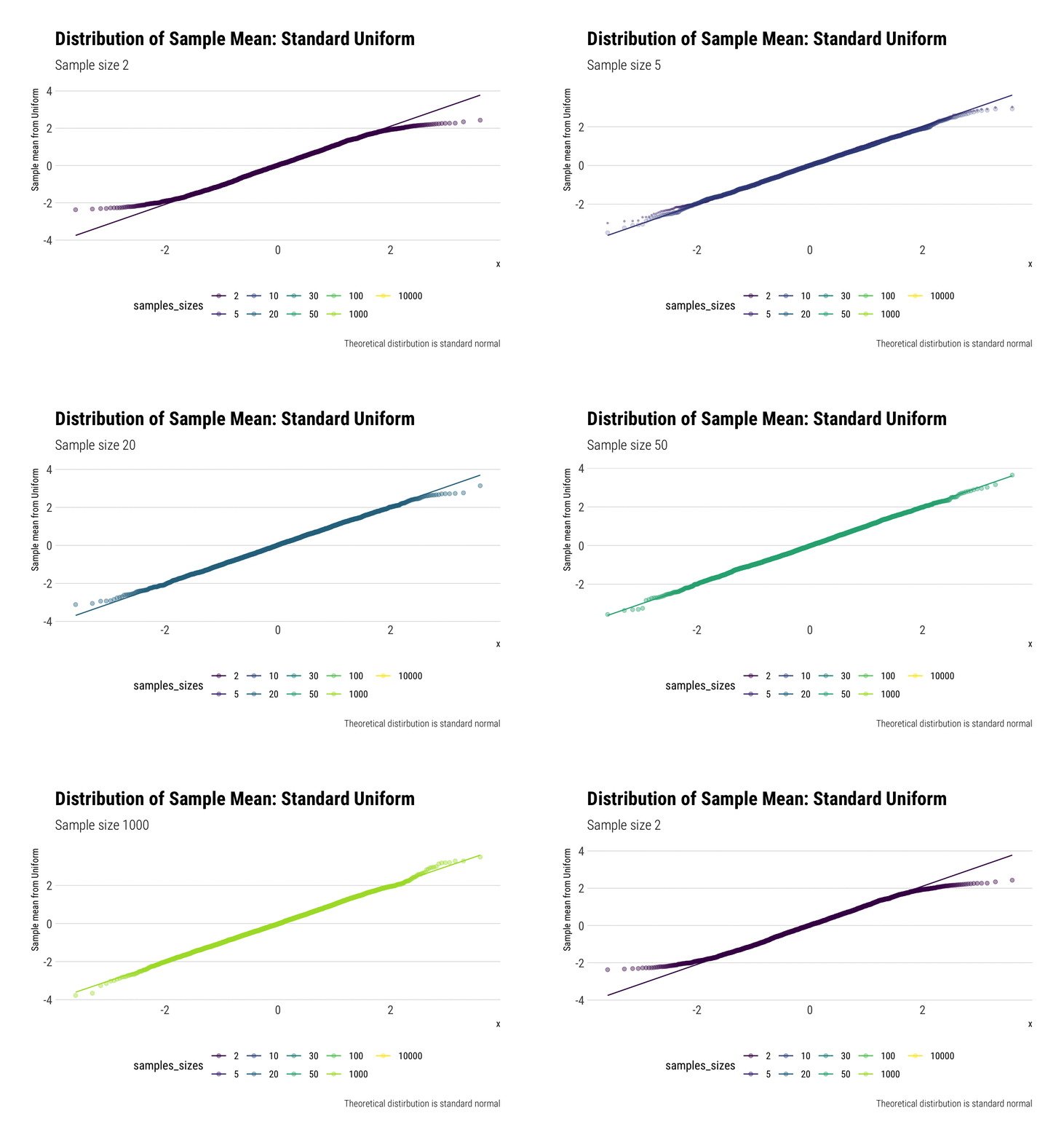

Now, for the densities:

uniform %>% 
  ggplot(aes(z, fill = samples_sizes)) +
  geom_density(aes(group = NA)) +
  transition_states(samples_sizes,
                    transition_length = 2,
    state_length = 1) +
  stat_function(fun = dnorm, aes(color = 'Normal'),
                         args = list(mean = 0, sd = 1),
                inherit.aes = FALSE) +
  enter_fade() +
  exit_shrink() +
  labs(subtitle = "Sample size {closest_state}",
       title = "Distribution of Sample Mean: Standard Uniform") +
  view_follow() -> uniform_dens
uniform_dens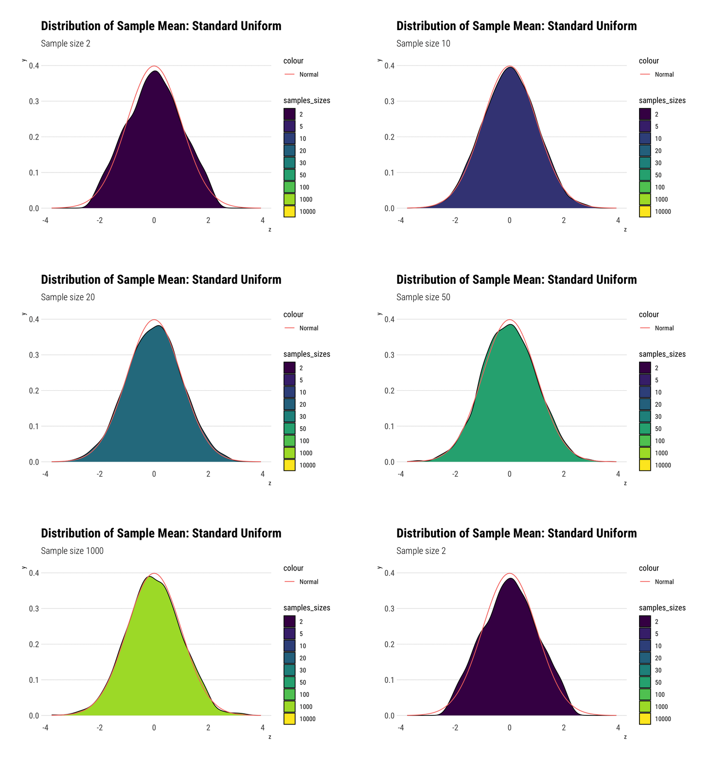

With \(n=5\) we already have a distribution extremely similar to a normal. That is, for the Standard Uniform, the CLT is useful even we have very few samples. We can confirm this by looking at the moments of the sample mean:

uniform %>% 
  group_by(samples_sizes) %>% 
  summarise(mean = mean(z),
            var = var(z),
            skew = mean(z^3),
            kurtosis = mean(z^4)) %>% 
  gt::gt() %>% 
  gt::fmt_number(vars(mean, var, skew, kurtosis))

samples_sizes	mean	var	skew	kurtosis
2	0.01	0.99	0.02	2.37
5	0.01	1.01	0.06	2.77
10	−0.01	0.97	−0.06	2.73
20	0.01	1.02	0.01	2.90
30	0.00	1.03	−0.02	3.16
50	−0.01	1.00	−0.01	2.97
100	−0.02	1.03	−0.06	3.37
1000	−0.01	1.02	−0.02	3.16
10000	−0.03	1.01	−0.04	2.95

Notice that, for higher moments, the LLN takes longer to be a valid approximation.

Semi-slow convergence: the exponential

Now, let’s do the same for the exponential (\(\lambda = 1\)). We calculate the \(Z\)-scores and then plot the comparisons. Let’s check the \(QQ\)-plot:

exponential <- simulate_sample_means(rexp, 3000, ns) %>% 
  rename(exponential = value) %>% 
  group_by(samples_sizes) %>% 
  mutate(z = (exponential - 1)*sqrt(samples_sizes)) %>% 
  ungroup() %>% 
  mutate(samples_sizes = factor(samples_sizes, ordered = TRUE))

exponential %>% 
  ggplot(aes(sample = z, color = samples_sizes)) +
  stat_qq(alpha = 0.4) +
  stat_qq_line(aes(group = NA)) +
  theme(legend.position = "bottom")  +
  transition_states(samples_sizes) +
  enter_fade() +
  exit_shrink() +
  view_follow() +
  labs(subtitle = "Sample size {closest_state}",
       title = "Distribution of Sample Mean: Exponential",
       caption = "Theoretical distirbution is standard normal",
       y = "Sample mean from Exponential")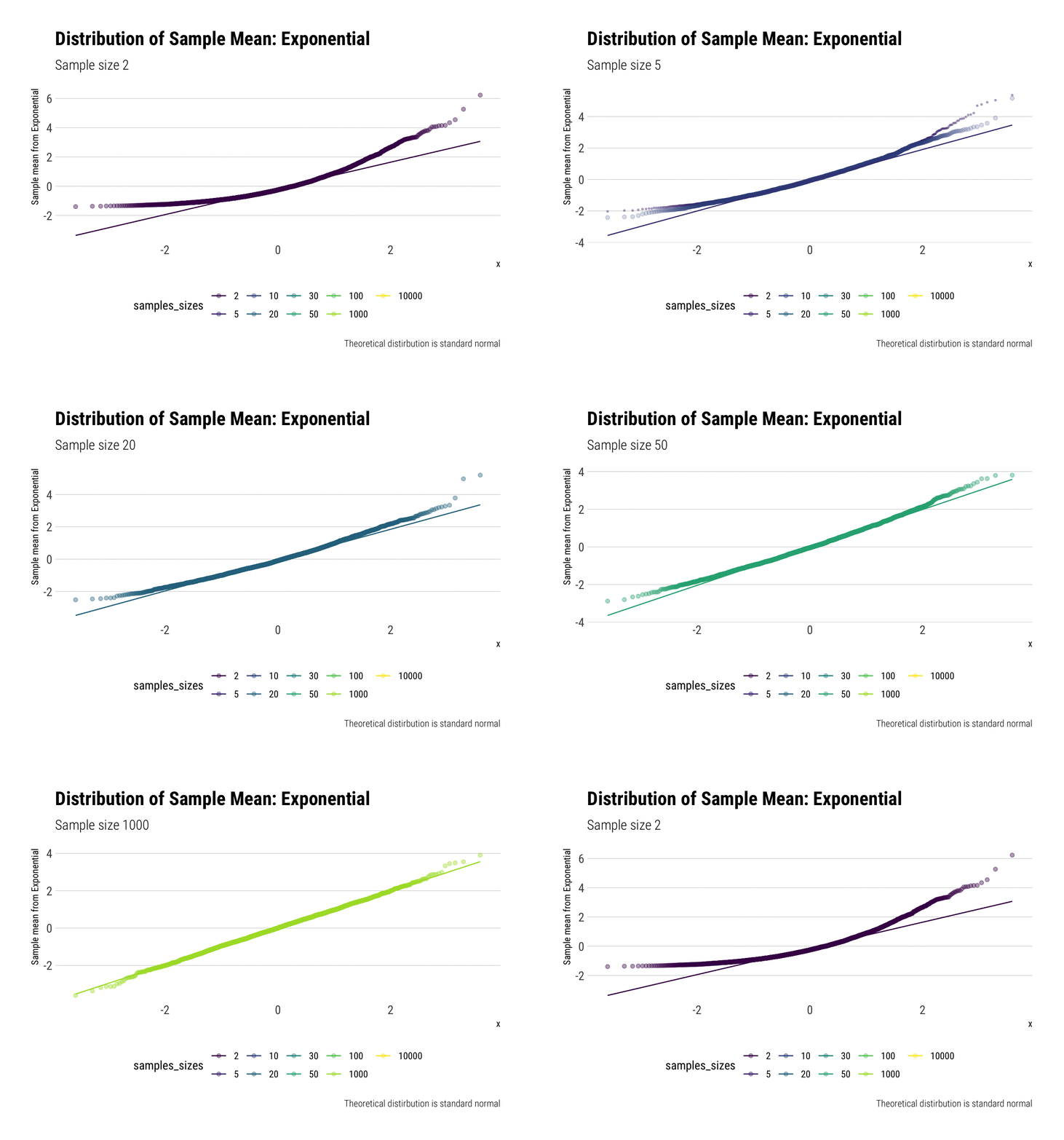

Now, for the densities:

exponential %>% 
  ggplot(aes(z, fill = samples_sizes)) +
  geom_density(aes(group = NA)) +
  transition_states(samples_sizes,
                    transition_length = 2,
    state_length = 1) +
  stat_function(fun = dnorm, aes(color = 'Normal'),
                         args = list(mean = 0, sd = 1),
                inherit.aes = FALSE) +
  enter_fade() +
  exit_shrink() +
  labs(subtitle = "Sample size {closest_state}",
       title = "Distribution of Sample Mean: Exponential",
       caption = "Theoretical distirbution is standard normal",
       y = "Sample mean from Exponential") +
  view_follow() -> exponential_dens
exponential_dens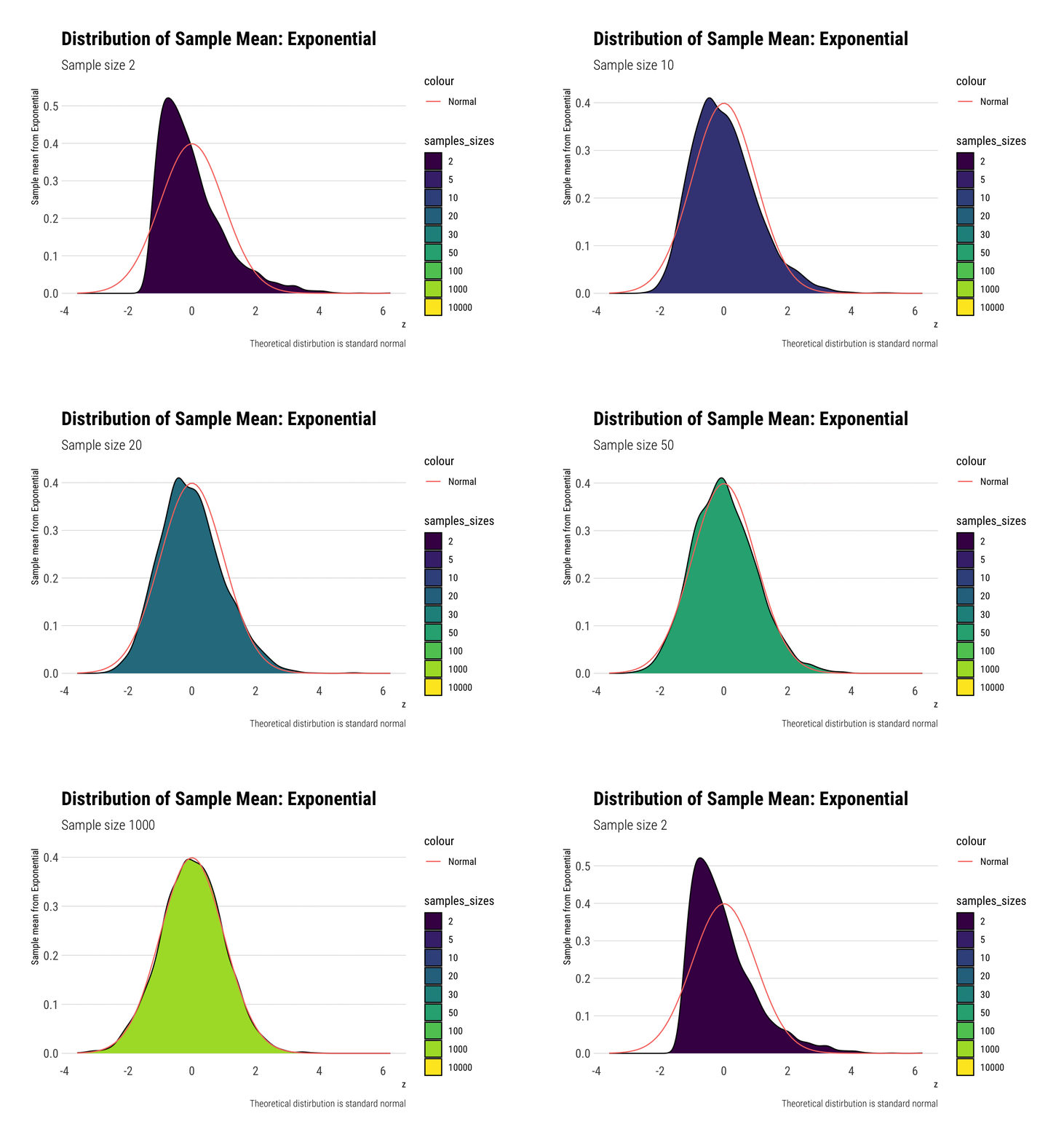

In comparison to the Standard Uniform, the convergence is slower with the Exponential: only with 20 or more observations there is a semblance of normality. However, that is still a totally achievable sample size. That is, the use of CLT is warranted with relatively few samples when we are working with an Exponential. We can confirm this by looking at the sample moments:

exponential %>% 
  group_by(samples_sizes) %>% 
  summarise(mean = mean(z),
            var = var(z),
            skew = mean(z^3),
            kurtosis = mean(z^4)) %>% 
  gt::gt() %>% 
  gt::fmt_number(vars(mean, var, skew, kurtosis))

samples_sizes	mean	var	skew	kurtosis
2	−0.02	0.99	1.30	5.20
5	0.01	1.04	1.05	4.88
10	0.03	1.00	0.65	3.43
20	−0.01	0.99	0.42	3.25
30	0.00	0.99	0.35	3.17
50	0.01	0.99	0.36	3.12
100	−0.02	1.02	0.21	3.24
1000	0.01	0.98	0.03	3.06
10000	0.01	1.02	0.03	2.91

Again, notice that, for higher moments, the LLN takes longer to be a valid approximation.

Leaving fast Convergence behind: Log Normal

With the lognormal, things start getting interesting. For a lognormal from an underlying standard normal, we need lots of observations to “see” the CLT. Let’s check the QQ-plot:

lognormal <- simulate_sample_means(rlnorm, 3000, ns) %>% 
  rename(lognormal = value) %>% 
  group_by(samples_sizes) %>% 
  mutate(z = (lognormal - exp(1/2) )/sqrt(( ( exp(1) - 1) * exp(1) ) / samples_sizes ) ) %>% 
  ungroup() %>% 
  mutate(samples_sizes = factor(samples_sizes, ordered = TRUE))

lognormal %>% 
  ggplot(aes(sample = z, color = samples_sizes)) +
  stat_qq(alpha = 0.4) +
  stat_qq_line(aes(group = NA)) +
  theme(legend.position = "bottom")  +
  transition_states(samples_sizes) +
  enter_fade() +
  exit_shrink() +
  view_follow() +
  labs(subtitle = "Sample size {closest_state}",
       title = "Distribution of Sample Mean: Lognormal",
       caption = "Theoretical distirbution is standard normal",
       y = "Sample mean from Lognormal")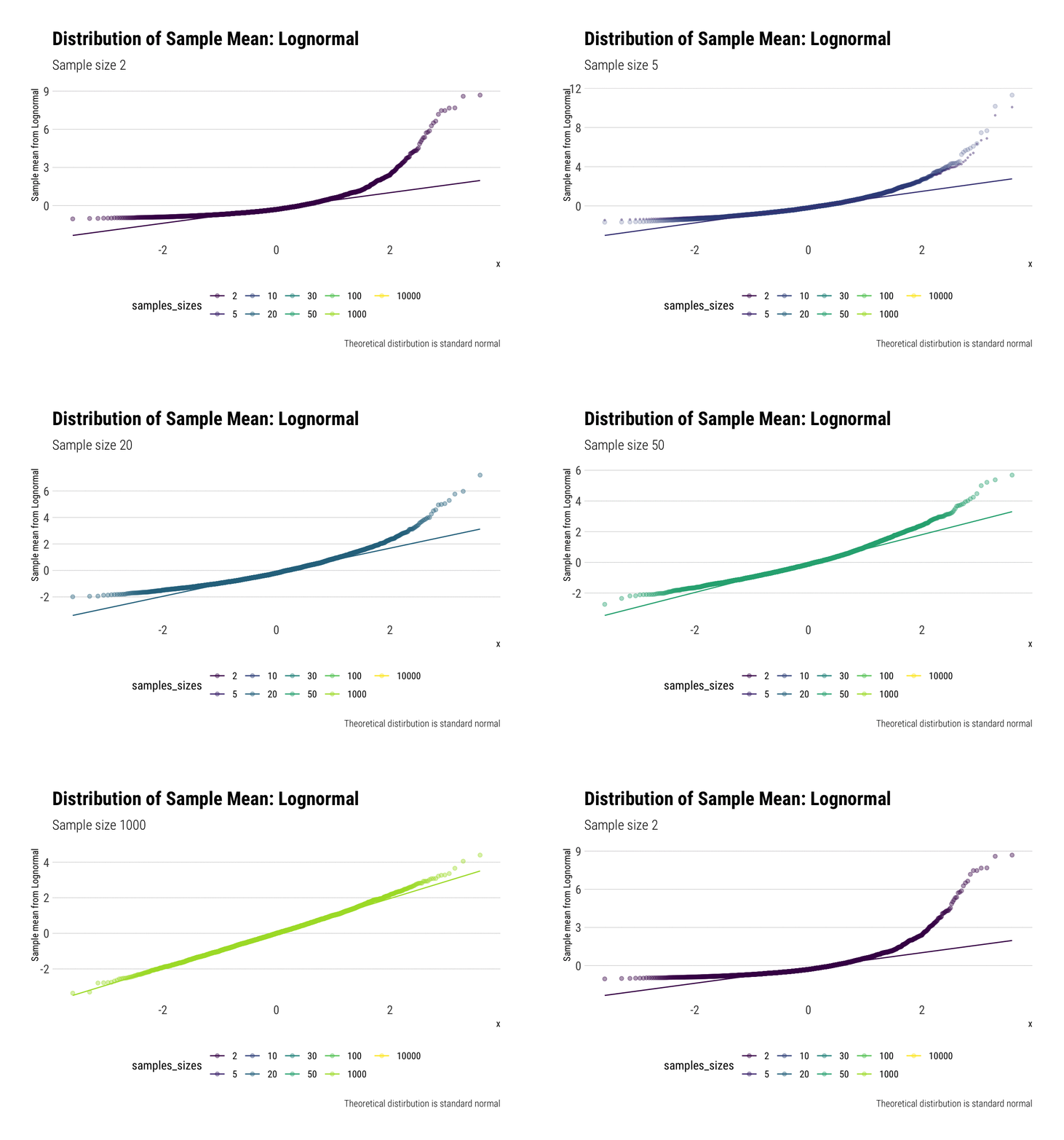

Now, for the densities:

lognormal %>% 
  ggplot(aes(z, fill = samples_sizes)) +
  geom_density(aes(group = NA)) +
  transition_states(samples_sizes,
                    transition_length = 2,
    state_length = 1) +
  stat_function(fun = dnorm, aes(color = 'Normal'),
                         args = list(mean = 0, sd = 1),
                inherit.aes = FALSE) +
  enter_fade() +
  exit_shrink() +
  view_follow() +
  labs(subtitle = "Sample size {closest_state}",
       title = "Distribution of Sample Mean: Lognormal",
       caption = "Theoretical distirbution is standard normal",
       y = "Sample mean from Lognormal") -> lognormal_dens
lognormal_dens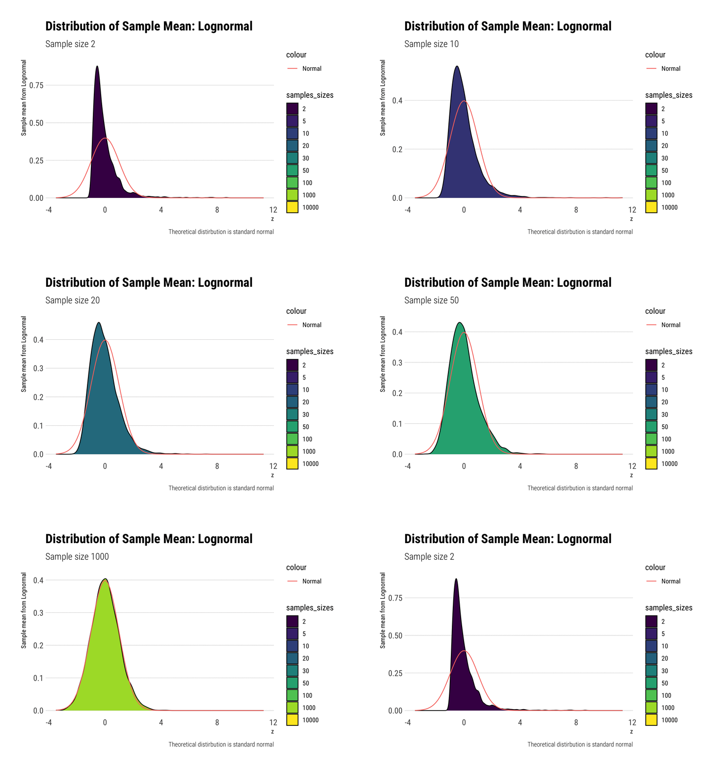

With the log-normal, the distribution does not look normal for any of the sample sizes. It takes a long-time for the distribution of the sample mean to lose its skeweness and it will take even longer for it to have the kurtosis of a standard normal:

lognormal %>% 
  group_by(samples_sizes) %>% 
  summarise(mean = mean(z),
            var = var(z),
            skew = mean(z^3),
            kurtosis = mean(z^4)) %>% 
  gt::gt() %>% 
  gt::fmt_number(vars(mean, var, skew, kurtosis))

samples_sizes	mean	var	skew	kurtosis
2	−0.03	0.88	2.70	16.19
5	0.00	0.96	2.12	12.57
10	0.01	1.10	2.69	18.36
20	−0.04	0.97	1.06	5.84
30	−0.03	0.94	0.78	4.01
50	0.01	1.05	0.97	4.93
100	0.01	0.92	0.43	2.94
1000	0.02	1.02	0.27	3.39
10000	0.02	1.00	0.11	3.15

Again, notice that, for higher moments, the LLN takes longer to be a valid approximation.

Worsening the problem

We can check how this problems exacerbate once we increase the variance of the underlying normal. For example, here it is a small change where \(sigma = 2\) for the underlying normal.

lognormal_large <- simulate_sample_means(function(x) rlnorm(n = x, sdlog = 2), 3000, ns) %>% 
  rename(lognormal = value) %>% 
  group_by(samples_sizes) %>% 
  mutate(z = (lognormal - exp(4/2) )/sqrt(( ( exp(4) - 1) * exp(4) ) / samples_sizes ) ) %>% 
  ungroup() %>% 
  mutate(samples_sizes = factor(samples_sizes, ordered = TRUE))

lognormal_large %>% 
  ggplot(aes(z, fill = samples_sizes)) +
  geom_density(aes(group = NA)) +
  transition_states(samples_sizes) +
  stat_function(fun = dnorm, aes(color = 'Normal'),
                         args = list(mean = 0, sd = 1),
                inherit.aes = FALSE) +
  enter_fade() +
  exit_shrink() +
  view_follow() +
  labs(subtitle = "Sample size {closest_state}",
       title = "Distribution of Sample Mean: Lognormal",
       caption = "Theoretical distirbution is standard normal",
       y = "Sample mean from Lognormal")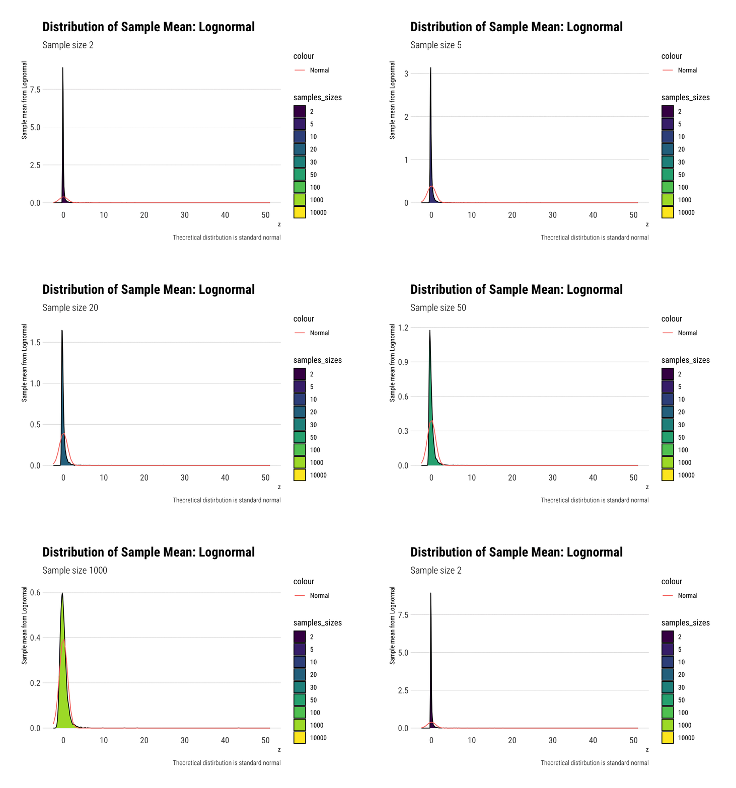

Indeed, now the sample mean’s distribution has a much longer right tail. That is, the skewness and kurtosis problems persists even at very large sample sizes.

lognormal_large %>% 
  group_by(samples_sizes) %>% 
  summarise(mean = mean(z),
            var = var(z),
            skew = mean(z^3),
            kurtosis = mean(z^4)) %>% 
  gt::gt() %>% 
  gt::fmt_number(vars(mean, var, skew, kurtosis))

samples_sizes	mean	var	skew	kurtosis
2	0.00	0.56	5.85	80.45
5	0.00	0.81	12.96	296.29
10	0.04	1.73	52.95	2,398.74
20	−0.03	0.65	6.83	137.13
30	0.03	1.18	20.64	609.30
50	−0.02	0.61	2.62	22.20
100	−0.01	0.72	3.49	38.18
1000	0.03	1.59	31.74	1,236.59
10000	0.01	0.86	0.78	4.35

Why does this happen? Because we have increased the importance of the tail in our calculations. Every once in a while we will get an extreme event: in the sample mean, this event can be averaged out. Here, even the square of the extreme event can be averaged out. However, this extreme event, when taking its cube or even its quartic value, cannot be so easily averaged out. To do so, we would need many, many more samples than we currently have.

Convergence before the sun dies? Pareto (alpha = 2.1)

We must remember that the CLT holds when the samples have finite variance. Therefore, we must pick a Pareto with a tail exponent larger than \(2\) (If you need a refresher on the intuitive meaning of the tail exponent, check this post ) In this case, we chose \(\alpha = 2.1\).

Let’s check the \(QQ\)-plot:

alpha <- 2.1
rpareto <- function(n) {
   (1/runif(n)^(1/alpha)) # inverse transform sampling
}

mean_pareto <- alpha / (alpha-1)
var_pareto <-  alpha / ((alpha-1)^2 * (alpha-2))

pareto <- simulate_sample_means(rpareto, 3000, ns) %>% 
  rename(pareto = value) %>% 
  group_by(samples_sizes) %>% 
  mutate(z = (pareto - mean_pareto )/sqrt( var_pareto / samples_sizes ) ) %>% 
  ungroup() %>% 
  mutate(samples_sizes = factor(samples_sizes, ordered = TRUE))

pareto %>% 
  ggplot(aes(sample = z, color = samples_sizes)) +
  stat_qq(alpha = 0.4) +
  stat_qq_line(aes(group = NA)) +
  theme(legend.position = "bottom")  +
  transition_states(samples_sizes) +
  enter_fade() +
  exit_shrink() +
  view_follow() +
  labs(subtitle = "Sample size {closest_state}",
       title = "Distribution of Sample Mean: Pareto (alpha = 2.1)",
       caption = "Theoretical distirbution is standard normal",
       y = "Sample mean from Pareto")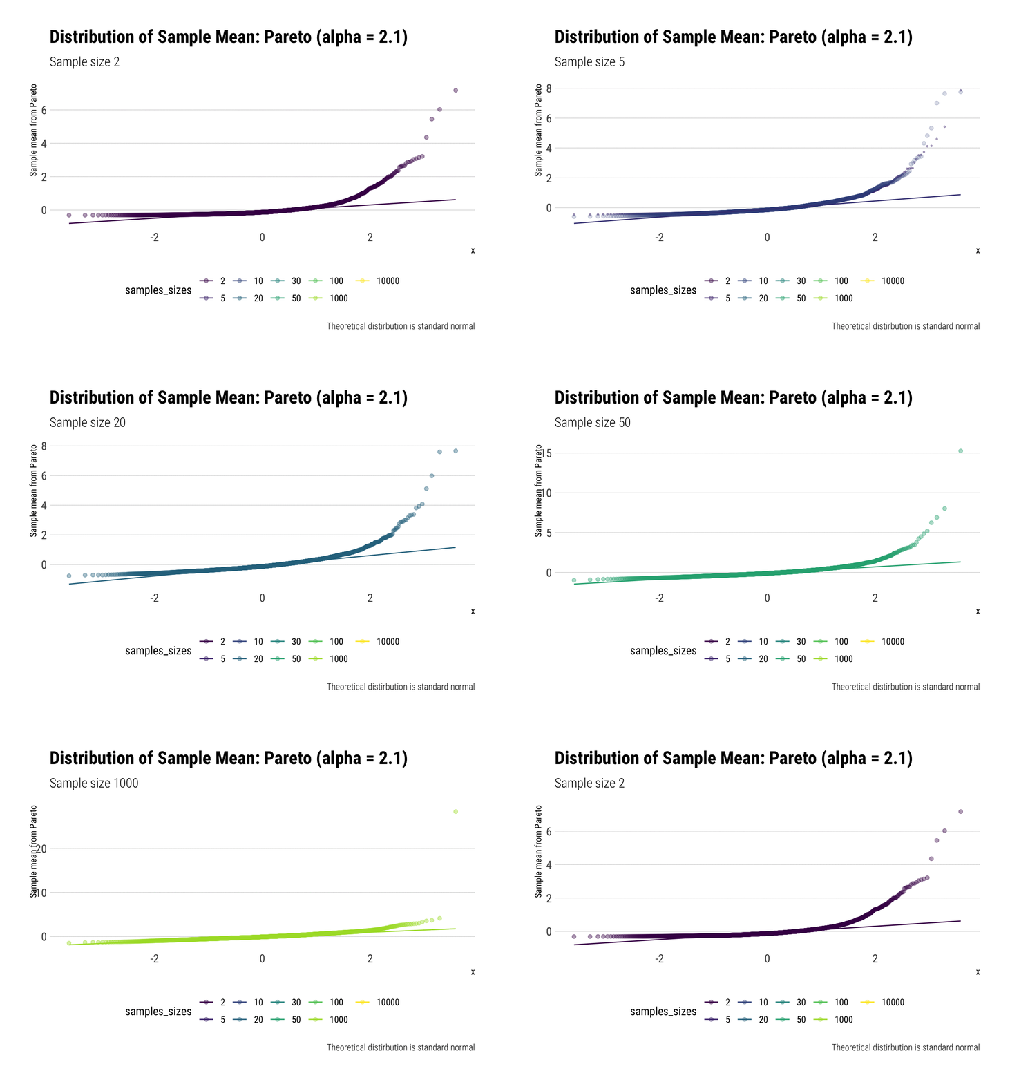

Now for the densities:

pareto %>% 
  ggplot(aes(z, fill = samples_sizes)) +
  geom_density(aes(group = NA)) +
  transition_states(samples_sizes,
                    transition_length = 2,
    state_length = 1) +
  stat_function(fun = dnorm, aes(color = 'Normal'),
                         args = list(mean = 0, sd = 1),
                inherit.aes = FALSE) +
  enter_fade() +
  exit_shrink() +
  view_follow() +
  labs(subtitle = "Sample size {closest_state}",
       title = "Distribution of Sample Mean: Pareto (alpha = 2.1)",
       caption = "Theoretical distirbution is standard normal",
       y = "Sample mean from Pareto") -> pareto_densities
pareto_densities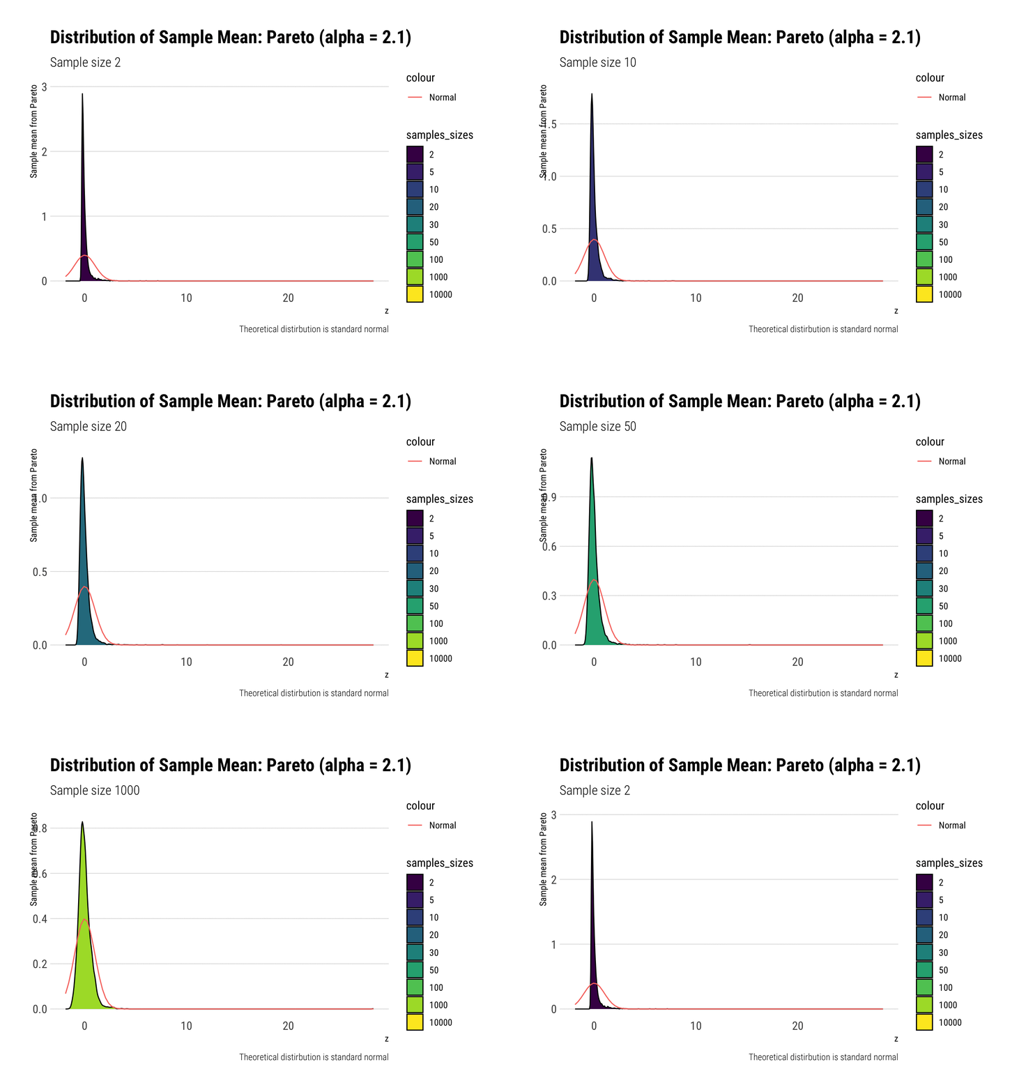

As it can be seen from the plot above, the distribution of a Pareto’s sample mean is very far from a normal, even with 10k in each sample. For one, its right-tail is very long. Also, the sample variance seems way too small. That is, although the first moment converges, the second does not: this is expected, specially with fat tails: the LLN works way too slowly. Notice, however, that it doesn’t make much sense to calculate the sample skewness nor kurtosis: their theoretical counterparts do not exist for the underlying random variable and neither exist for its sample mean estimator.

pareto %>% 
  group_by(samples_sizes) %>% 
  summarise(mean = mean(z),
            var = var(z)) %>% 
  gt::gt() %>% 
  gt::fmt_number(vars(mean, var))

samples_sizes	mean	var
2	0.00	0.20
5	−0.01	0.21
10	−0.02	0.26
20	−0.01	0.29
30	0.00	0.47
50	0.01	0.43
100	0.00	0.33
1000	0.01	0.63
10000	0.01	0.82

This is what fat-tails do to you. Even when their theoretical moments do exist, their very, very long pre-asymptotic behavior invalidate the use of both LLN and CLT for any reasonable amount of data The intuition for the under-estimation of the variance is simple: a large part of its theoretical variance comes from the tail; however, it takes a lot, a lot, of data to “see” the tail. Therefore, our sample won’t be able to measure correctly the variance because we don’t have enough data to see the tail.

More forgiving Pareto

Notice that as the Pareto’s tail exponent increases, these problems are mitigated. For example, let’s take a Pareto with \(\alpha = 4.1\) such that both skewness and kurtosis exist:

alpha <- 4.1

mean_pareto <- alpha / (alpha-1)
var_pareto <-  alpha / ((alpha-1)^2 * (alpha-2))

pareto_forgiving <- simulate_sample_means(rpareto, 3000, ns) %>% 
  rename(pareto = value) %>% 
  group_by(samples_sizes) %>% 
  mutate(z = (pareto - mean_pareto )/sqrt( var_pareto / samples_sizes ) ) %>% 
  ungroup() %>% 
  mutate(samples_sizes = factor(samples_sizes, ordered = TRUE))

pareto_forgiving %>% 
  ggplot(aes(z, fill = samples_sizes)) +
  geom_density(aes(group = NA)) +
  transition_states(samples_sizes) +
  stat_function(fun = dnorm, aes(color = 'Normal'),
                         args = list(mean = 0, sd = 1),
                inherit.aes = FALSE) +
  enter_fade() +
  exit_shrink() +
  view_follow() +
  labs(subtitle = "Sample size {closest_state}",
       title = "Distribution of Sample Mean: Pareto (alpha = 4.1)",
       caption = "Theoretical distirbution is standard normal",
       y = "Sample mean from Pareto")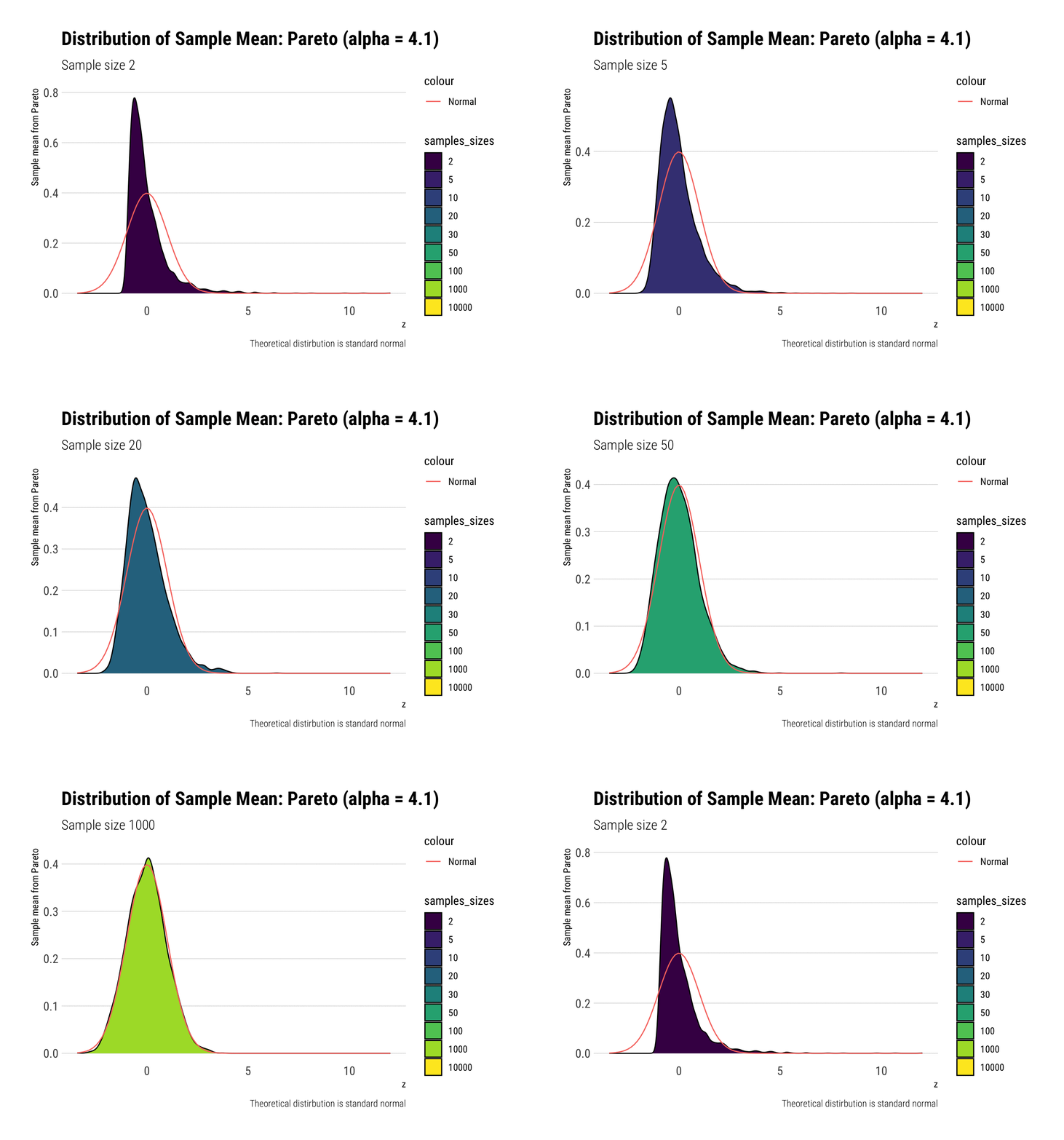

As it can be seen, the problems with the tail diminish as we increase the tail exponent. We can also check the convergence of higher moments:

pareto_forgiving %>% 
  group_by(samples_sizes) %>% 
  summarise(mean = mean(z),
            var = var(z),
            skewness = mean(z^3),
            kurtosis = mean(z^4)) %>% 
  gt::gt() %>% 
  gt::fmt_number(vars(mean, var, skewness, kurtosis))

samples_sizes	mean	var	skewness	kurtosis
2	0.01	0.97	3.26	23.69
5	−0.02	0.88	1.58	8.07
10	0.01	0.93	1.18	5.27
20	0.00	0.95	0.94	4.28
30	0.04	1.04	1.62	11.86
50	0.01	0.97	0.75	4.64
100	0.00	0.96	0.53	3.34
1000	0.00	0.96	0.12	2.75
10000	0.00	1.00	−0.05	3.06

Conclusion

In theory, the CLT is a valid approximation for the distribution of the sample mean: fat-tails (with finite variance) included. However, the CLT only tells us the final destination of the convergence: it does not say anything regarding how fast this convergence will be. As our Monte-Carlo experiments have shown, this convergence can be extremely slow: so slow, that the use of the CLT as a valid approximation may not be warranted at all for our usual samples sizes.

Reuse

https://creativecommons.org/licenses/by/4.0/